

Fluid Mechanics in Real Plants: Why Experience Favors Safety Margins
In chemical engineering, there is a big difference between how fluids behave in textbooks and how they behave inside an operating plant.
At ChemEngZone, our perspective comes straight from day-to-day experience on the plant floor—not from trying to be math geniuses. When you spend time around real equipment, you quickly learn that operating conditions fluctuate, piping layouts are complex, and process mixtures rarely behave like ideal models. That hands-on reality teaches you one fundamental rule: whenever you make operational or safety decisions, you have to stay conservative.
Looking at the physics behind fluid motion, from basic shear stress and rheology up to the Navier-Stokes equations, shows how complex real fluids can be when they move. When you cannot predict every variable on paper, we like to leave you with one piece of process safety advice to follow whenever possible: always choose conservative solutions.
The Nature of Fluids: Shear Stress and the No-Slip Condition
To understand how a fluid behaves inside a pipe or a piece of chemical equipment, we have to start with its true physical definition. Physics defines a fluid as a substance that undergoes continuous deformation when subjected to a shear stress (τ).
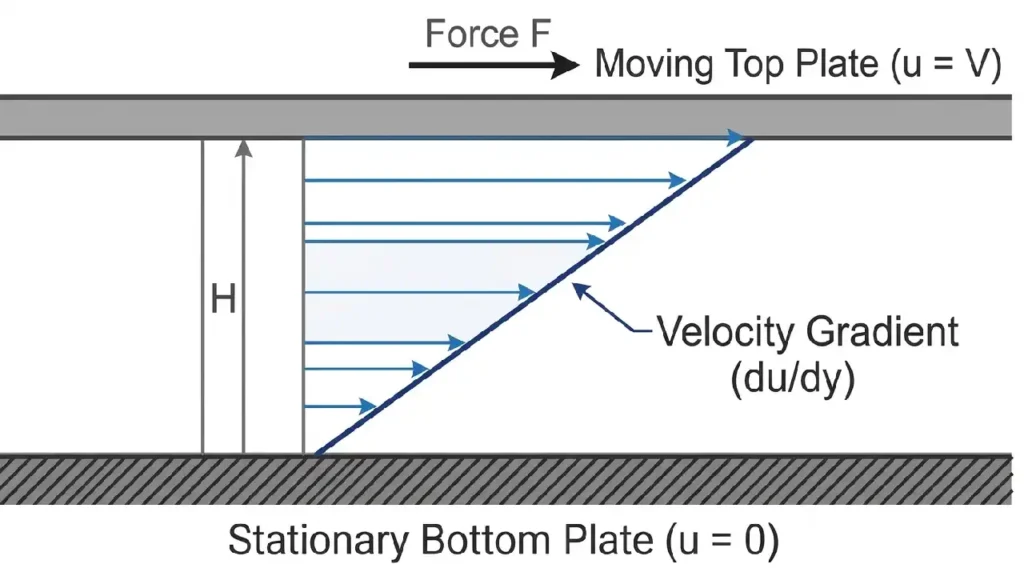
Consider the classic rheology experiment: a fluid is bounded by two large parallel plates separated by a tiny distance H. The bottom plate is held completely fixed, while a force F is applied to the upper plate, causing it to move at a constant velocity V. Unlike a solid (which would bend slightly under a force, hit a finite deformation, and stop), a fluid will continue to deform and flow for as long as that force is applied.
From this experiment, two fundamental concepts for Transport Phenomena are born:
- Shear Stress (τ = F/A): The force per unit area exerted on the fluid.
- The No-Slip Condition: Because of friction at the solid boundaries, the fluid bounding the lower fixed plate has zero velocity, while the fluid bounding the upper plate moves exactly at the plate’s velocity V.
This velocity gradient established across the gap (du/dy) defines the Shear Rate (γ̇), which represents the rate of fluid deformation and is reported in units of reciprocal seconds (s⁻¹).
The Rheology Map: Fluid Models vs. Plant Reality
In fluid mechanics, an ideal fluid assumes zero viscosity and zero internal friction. You can safely use this approximation for quick estimates with low-viscosity gases or short, low-velocity lines where friction losses are negligible. In most real process lines, however, fluids have measurable viscosity, meaning internal friction and pressure drops cannot be ignored.
To quantify that internal friction, the ratio of shear stress to shear rate defines the single most critical physical property in your piping: viscosity (μ).
The SI units of absolute (or shear) viscosity are kg/(m · s) or Pa · s (Pascal-seconds). The cgs unit (an older metric system still widely used in industry) for viscosity is the poise (P), where:
1 Pa·s = 10 P = 1000 centipoise (cP) = 0.672 lbm/(ft·s)
In standard fluid mechanics, the terms dynamic viscosity, absolute viscosity, and shear viscosity all refer to the same property (μ). In practical terms, this property measures a fluid’s internal resistance to motion. Inside a real plant, that single resistance affects almost everything, from piping pressure drops and pump sizing to heat transfer rates in heat exchangers and mixing efficiency in reactors.
Alongside dynamic viscosity, engineers also frequently use kinematic viscosity (ν), defined as the ratio of dynamic viscosity to fluid density, which represents the fluid’s resistance to flow relative to its inertia:
The SI units of kinematic viscosity are m²/s, while the cgs unit is the stoke (St), where 1 St = 1 cm²/s. In everyday plant practice, you will most commonly see this reported in centistokes (cSt).
Rheology studies this exact relationship, allowing us to map industrial fluids into distinct categories:
- Newtonian Fluids: These are the straightforward fluids of linear engineering (water, gases, low-molecular-weight solvents). For a Newtonian fluid, viscosity remains constant regardless of how fast you stir, mix, or pump it. Newton’s law of viscosity is simply written as:
- Non-Newtonian Fluids: In real chemical processes, Newtonian behavior is often the exception rather than the rule. Polymer melts, paints, concentrated suspensions, and heavy sludges exhibit an apparent viscosity that varies with the shear rate.
- Bingham Plastics: Highly concentrated suspensions (like column bottom sludges) that require a definitive threshold stress, called a yield stress , before any continuous deformation and flow can even begin.
- Shear-Thinning (Pseudoplastic): Fluids whose apparent viscosity decreases as the shear rate increases, commonly fitted to a power-law model.
- Bingham Plastics: Highly concentrated suspensions (like column bottom sludges) that require a definitive threshold stress, called a yield stress , before any continuous deformation and flow can even begin.
Scaling Up to Momentum Balances: Cauchy and Navier-Stokes
Once you know how a real fluid handles internal friction, you need a way to calculate how it moves through an entire piping network. At this point, a simple mechanical energy balance is no longer enough.
As seen in Bernoulli’s Principle: Equation & Applications, the classic Bernoulli equation treats the fluid as ideal—completely ignoring viscosity and internal friction. To account for real viscous losses in a plant line, engineers have to shift from an energy balance to a true force balance: the conservation of linear momentum.
The starting point for this balance is the Cauchy momentum equation, which describes how momentum is conserved in any continuous material—whether it is water, gas, molten polymer, or a heavy sludge:
The Cauchy equation is a magnificent universal law, but it leaves the internal friction term—the stress tensor entirely open, so that it can be calculated using a specific constitutive equation for each type of fluid.
When we specialize Cauchy’s universal skeleton by assuming the fluid is strictly incompressible, Newtonian, and possesses a constant viscosity (μ), we can substitute Newton’s specific viscous law into the equation. Crunching the math yields the definitive Navier-Stokes equation:
In this single expression, the inertial terms on the left-hand side (representing the forces driving the fluid forward) battle directly against the viscous terms on the right-hand side (representing the internal friction driven by viscosity).
Plant Floor Realities and the Breaking Point of Equations
On paper, Navier-Stokes is a complete, second-order differential equation. In theory, all you need to do is set your boundary conditions such as zero velocity at the pipe wall (no-slip) or zero shear stress at a liquid-gas interface, and let Computational Fluid Dynamics (CFD) software solve the rest.
In real plant operations, however, that neat mathematical picture quickly runs into practical limits:
- Turbulent Flow (Re > 4000): Industrial piping almost always operates in the turbulent regime. Solving the raw Navier-Stokes equations to capture every tiny eddy and swirl requires massive computing power that isn’t practical for everyday engineering. Instead, CFD tools rely on Reynolds-Averaged Navier-Stokes (RANS) models, which simplify the problem by introducing Reynolds stresses—approximations calibrated through experimental correlations rather than pure theory.
- Two-Phase Critical Flows: When sizing relief lines or pressure safety valves (PSVs) that vent a boiling liquid and gas mixture at the same time, standard single-phase equations break down. The liquid-gas interface shifts constantly, and predicting pressure drop and momentum transfer requires specialized empirical correlations and hybrid models.
- Non-Newtonian Fluids: The moment your process fluid stops behaving like a simple Newtonian liquid, the standard Navier-Stokes equation no longer applies. You have to step back to Cauchy’s general momentum equation and plug in dedicated rheological models, such as Herschel-Bulkley or Ostwald-de Waele, to describe how viscosity changes under shear.
Conclusion
Tracing fluid mechanics from basic viscosity up to Navier-Stokes shows a clear pattern: the closer we get to real plant conditions, the more complex the math becomes. Once turbulence, two-phase mixtures, or thick sludges enter the picture, even advanced models rely on approximations.
Pure theory is valuable for understanding the physics behind flow and friction, yet it cannot capture every fluctuation in a live process. Based on hands-on experience in industrial facilities, ChemEngZone recommends pairing that physical understanding with field awareness, and always applying conservative safety margins to keep the plant running safely.
⬆️ Back to TopFluid Mechanics & Navier-Stokes Quiz
When sizing piping or relief systems in a real chemical plant, why do engineers rely on field experience and conservative safety margins rather than solving raw Navier-Stokes equations alone?
Other Articles You May Find Useful
- Fluid Dynamics Basics for Engineers
- The Law of Poiseuille and Laminar Pipe Flow
- Darcy-Weisbach Equation Explained
- Chemical Engineer Skills: 2 Field Practices
Useful External References
- NASA Glenn Research Center – Navier-Stokes Equations
Clear technical overview of how the Navier-Stokes equations govern viscous fluid flow and why numerical approximations are needed in real-world applications.