Fluid Dynamics Basics for Engineers

Fundamental Concepts Governing Fluid Flow

Fluid dynamics explains how fluids move, how pressure changes along a flow system, and why velocity increases or decreases when geometry changes. In this context, a flow system may be a pipe, a duct, a channel, or any connected path through which the fluid is transported.

In chemical engineering, fluid dynamics is applied to fluid transport operations, that is, the handling, distribution, and control of fluids within industrial plants. These are fundamental unit operations, because every process depends in some way on moving fluids from one point to another under controlled conditions.

Ideal Flow as the Reference Model

Fluid dynamics is introduced by moving from simple models to more complex ones. The starting point is the steady motion of an ideal incompressible fluid, where viscous effects are neglected.

Although this model does not describe real fluids in a strict sense, it provides a clear reference framework. It allows the main conservation principles to be introduced without the additional complications associated with viscosity, compressibility, or turbulence.

Within this ideal-flow framework, several concepts are introduced that remain central to all subsequent analyses:

• streamlines and flow tubes, used to describe the geometry of fluid motion;
• flow rate and the continuity equation, expressing mass conservation;
• Bernoulli’s equation, relating pressure, velocity, and elevation in energetic terms.

These concepts are first established under ideal conditions and then extended to more realistic situations, where additional effects must be considered.

Steady Motion of Fluids

The simplest type of fluid motion to analyze is steady flow.

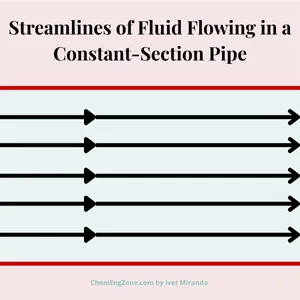
A flow is steady when the fluid properties at a given point do not change with time.

If a fixed point is considered inside the conduit, every particle passing through that point has the same velocity, pressure, and density. These properties may vary from one location to another, but at each point they remain constant over time.

Figure 1 shows this situation in a constant-section pipe. The lines representing the fluid motion, called streamlines, are parallel and equally spaced, indicating that the flow pattern remains unchanged along the conduit.

Under these conditions, two fundamental ideas can be established: the flow field is stable in time, and fluid motion can be represented by streamlines tangent to the local velocity vector.

Streamlines and Flow Tubes

Streamlines can be visualized experimentally by adding dye to a liquid flow or introducing lightweight tracer particles. These tracers reveal how fluid particles align with the velocity field inside a conduit.

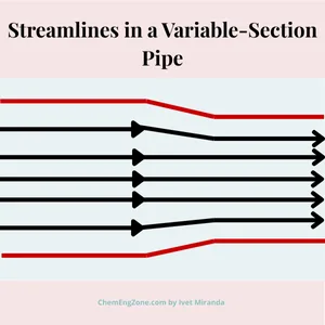
Figure 2 shows the case of a variable–section pipe. Here the streamlines are no longer parallel:

• they become denser where the pipe narrows, indicating higher velocity;
• they spread out where the pipe widens, indicating lower velocity.

This simple observation anticipates the principle of continuity: if the same amount of fluid passes through every section of the pipe, then velocity must increase when the cross–section decreases, and vice versa.

When a family of streamlines passes through the points of a closed curve, they form what is called a flow tube. A flow tube behaves as if it were a real conduit: no fluid crosses its boundaries, and the flow remains entirely confined inside.

Flow Rate and the Continuity Equation

Once the concept of a stream tube is introduced, it is possible to define flow rate.

In the context of fluid dynamics, this quantity represents the volume of fluid that crosses a section of the conduit in a given unit of time.

The idea is simple: consider the volume of fluid contained in a stream tube as it passes through a cross–section in a given unit of time.

For a section S and an average velocity v, the volumetric flow rate is: Q=S⋅v

where:

• Q = volumetric flow rate [m3/s][
• S = cross–sectional area [m2]
• v= average velocity across the section [m/s]

In steady incompressible flow, the volumetric flow rate is the same at every section of the conduit. This condition is expressed by the continuity equation: S1 v1=S2 v2, which shows that velocity is inversely proportional to the cross–sectional area.

Continuity in a Variable-Section Pipe

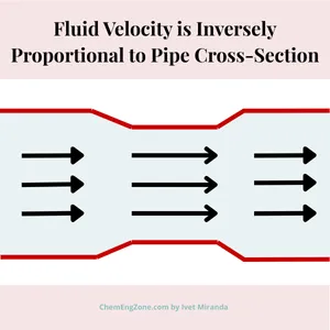
In Figure 4, two sections of the pipe are compared:

• At section 1, the fluid has cross–sectional area S1​ and velocity v1.
• At section 2, the fluid has cross–sectional area S2 and velocity v2.

Because the volumetric flow rate must remain constant in steady incompressible flow, the following condition applies: S1v1=S2v2

This equation shows that velocity is inversely proportional to the cross–sectional area. In other words, the fluid accelerates when the pipe narrows and slows down when the pipe widens.

Pressure–Velocity Relationship in Steady Flow

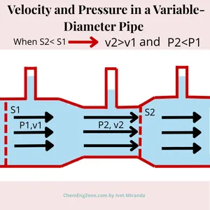
The continuity equation explains that velocity must increase when the cross–section of a pipe decreases. However, experiments with manometers show an additional effect: the static pressure in the constricted region becomes lower than in the wider region.

Figure 5 illustrates this result.

At section 1, the fluid has cross–section S1​, velocity v1​, and pressure P1​. At section 2, where the pipe narrows to S2​, the velocity increases to v2​ while the static pressure drops to P2​.

S2<S1⇒ v2>v1 and P2<P1.

In fluid dynamics, this observation is fundamental because it prepares the ground for the general relation between pressure, velocity, and elevation: Bernoulli’s equation.

Conclusion

These fundamental observations show that velocity, pressure, and geometry are inherently linked in fluid motion.

At this stage, fluid dynamics provides the descriptive tools needed to understand how a flow behaves when conditions change.

The energetic interpretation that explains why these changes occur belongs to the next step of fluid mechanics, where pressure, velocity, and elevation are analysed as different forms of mechanical energy carried by the fluid.

⬆️ Back to Top

Other Articles You May Find Useful

• Bernoulli’s Principle: Equation & Applications
• Bernoulli Principle Example: Venturi Meter
• The Law of Poiseuille and Laminar Pipe Flow
• Unit Operations in Chemical Engineering: Types and Examples
• Chemical Engineering Core Disciplines – A Practical Overview

FAQ